Reading, filtering and visualizing geospatial vector data
This tutorial is based on a similar one for R and shows how simpler and cleanly we can do this in Julia with GMT.jl. Vector data are composed of discrete geometric locations (x, y values) known as vertices that define the “shape” of the spatial object. There are three types of vector data: Points, Lines and Polygons (see more at, for example, GIS in Python). Geospatial vector data is often stored in the shapefile format and that is the format that we will use is this tutorial, but other formats could have been used without fundamental changes to the procedures shown below.
Reading vector data
Read a shapefile representing Colombian departments which has been previously downloaded from DIVA-GIS, and not forgetting to load the package first.
using GMT
deptos = gmtread(GMT.TESTSDIR * "COL_adm1.shp.zip");
We can see what the contents of the deptos object are, but because there are many polygons we will restrict to show only the first 7 from the attribute table. For that we use the info function that plots several types of information depending on the input data type. For GMTdatasets the attribs keyword lets us limit the number of table rows that are printed.
info(deptos, attribs=7)

Attribute table (Dict{String, String})
┌─────┬───────────┬──────┬─────────────┬───────────┬─────┬──────┬──────────────┬──────────┬───────────┐
│ Row │ NAME_1    │ ID_1 │ ENGTYPE_1   │ NL_NAME_1 │ ISO │ ID_0 │ TYPE_1       │ NAME_0   │ VARNAME_1 │
├─────┼───────────┼──────┼─────────────┼───────────┼─────┼──────┼──────────────┼──────────┼───────────┤
│   1 │ Amazonas  │ 1    │ Commissiary │           │ COL │ 53   │ Comisaría    │ Colombia │           │
│   2 │ Amazonas  │ 1    │ Commissiary │           │ COL │ 53   │ Comisaría    │ Colombia │           │
│   3 │ Antioquia │ 2    │ Department  │           │ COL │ 53   │ Departamento │ Colombia │           │
│   4 │ Antioquia │ 2    │ Department  │           │ COL │ 53   │ Departamento │ Colombia │           │
│   5 │ Antioquia │ 2    │ Department  │           │ COL │ 53   │ Departamento │ Colombia │           │
│   6 │ Arauca    │ 3    │ Intendancy  │           │ COL │ 53   │ Intendencia  │ Colombia │           │
│   7 │ Atlántico │ 4    │ Department  │           │ COL │ 53   │ Departamento │ Colombia │           │
└─────┴───────────┴──────┴─────────────┴───────────┴─────┴──────┴──────────────┴──────────┴───────────┘
It is always useful to know the coordinate reference system of the data object. For that we will use again the info function, but this time with the crs keyword.
info(deptos, crs=true)

PROJ: +proj=longlat +datum=WGS84 +no_defs
WKT: GEOGCS["WGS 84",
    DATUM["WGS_1984",
        SPHEROID["WGS 84",6378137,298.257223563]],
    PRIMEM["Greenwich",0],
    UNIT["degree",0.0174532925199433]]
A fundamental starting point to understand data is to plot it. GMT can do it with great simplicity.
viz(deptos)
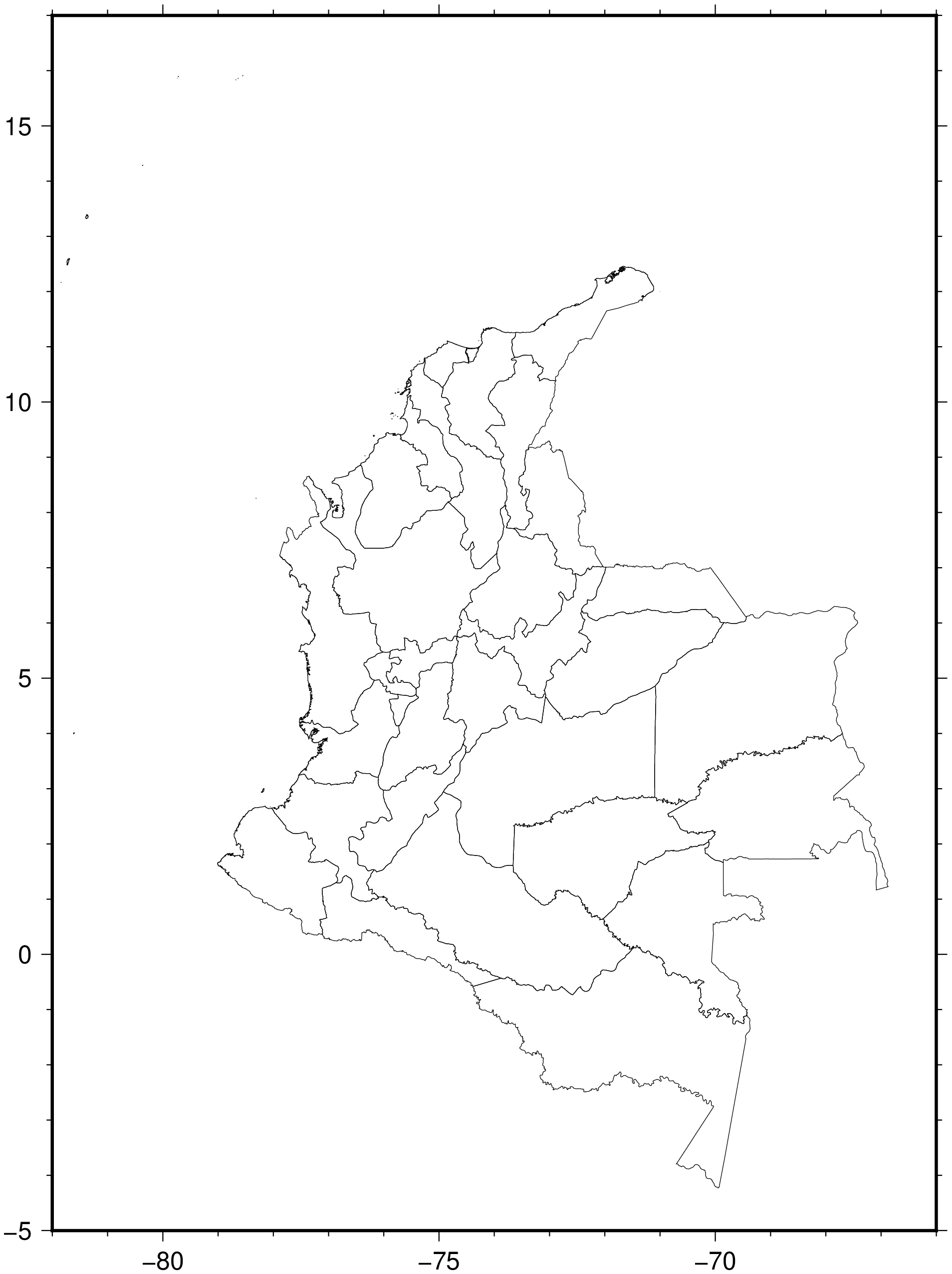
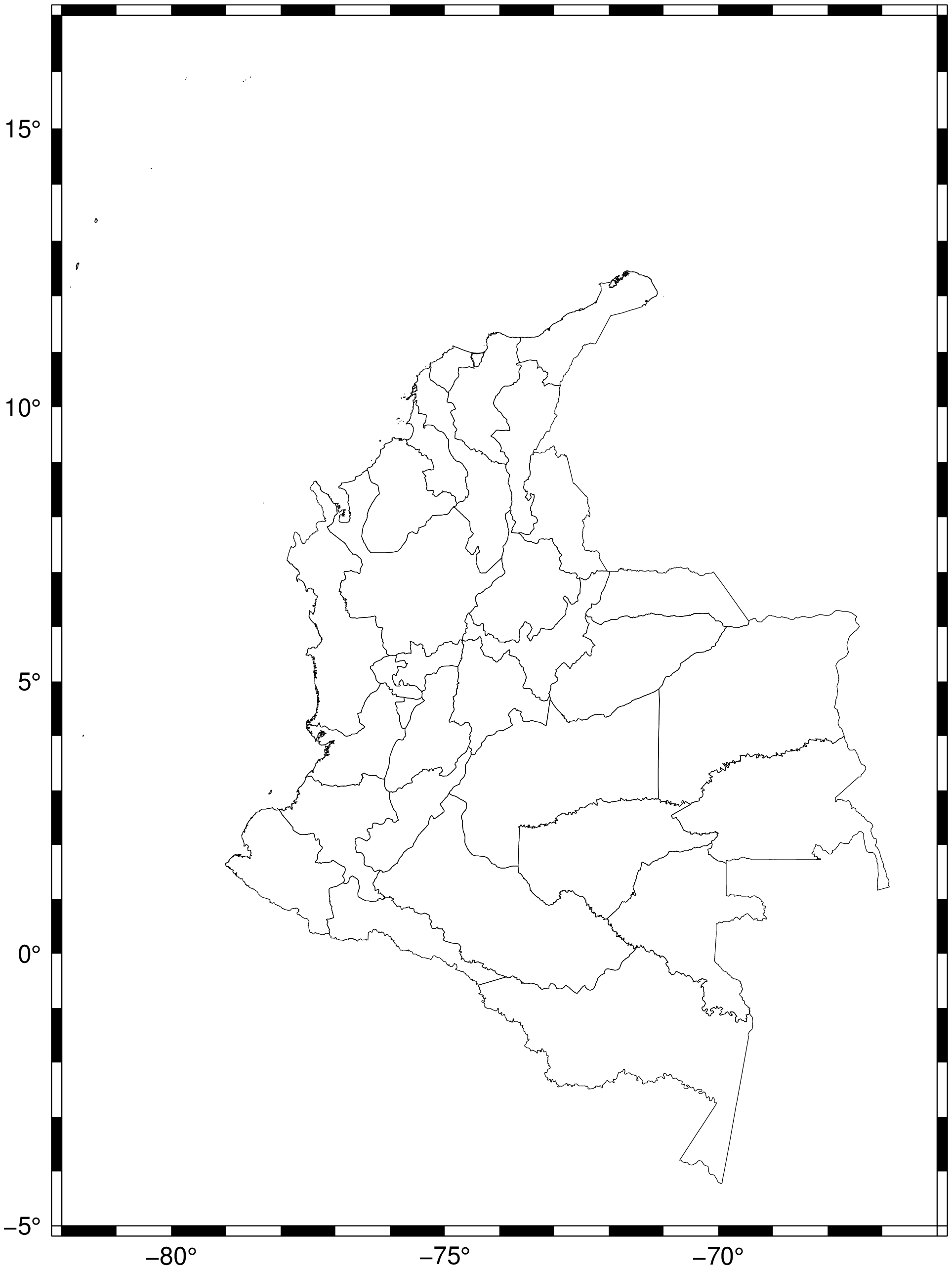
The somewhat large blank part on the upper part of the figure is due to small islands that are barely visible at this scale but also due to the automatic determination of the region boundaries. Also, since Colombia is close to equator the deformation implied by plotting geographical coordinates is not easily visible, but we can do better. We can tell GMT to guess a good projection for this region and automatically apply it.
viz(deptos, proj=:guess)
Filtering geospatial data based on attributes
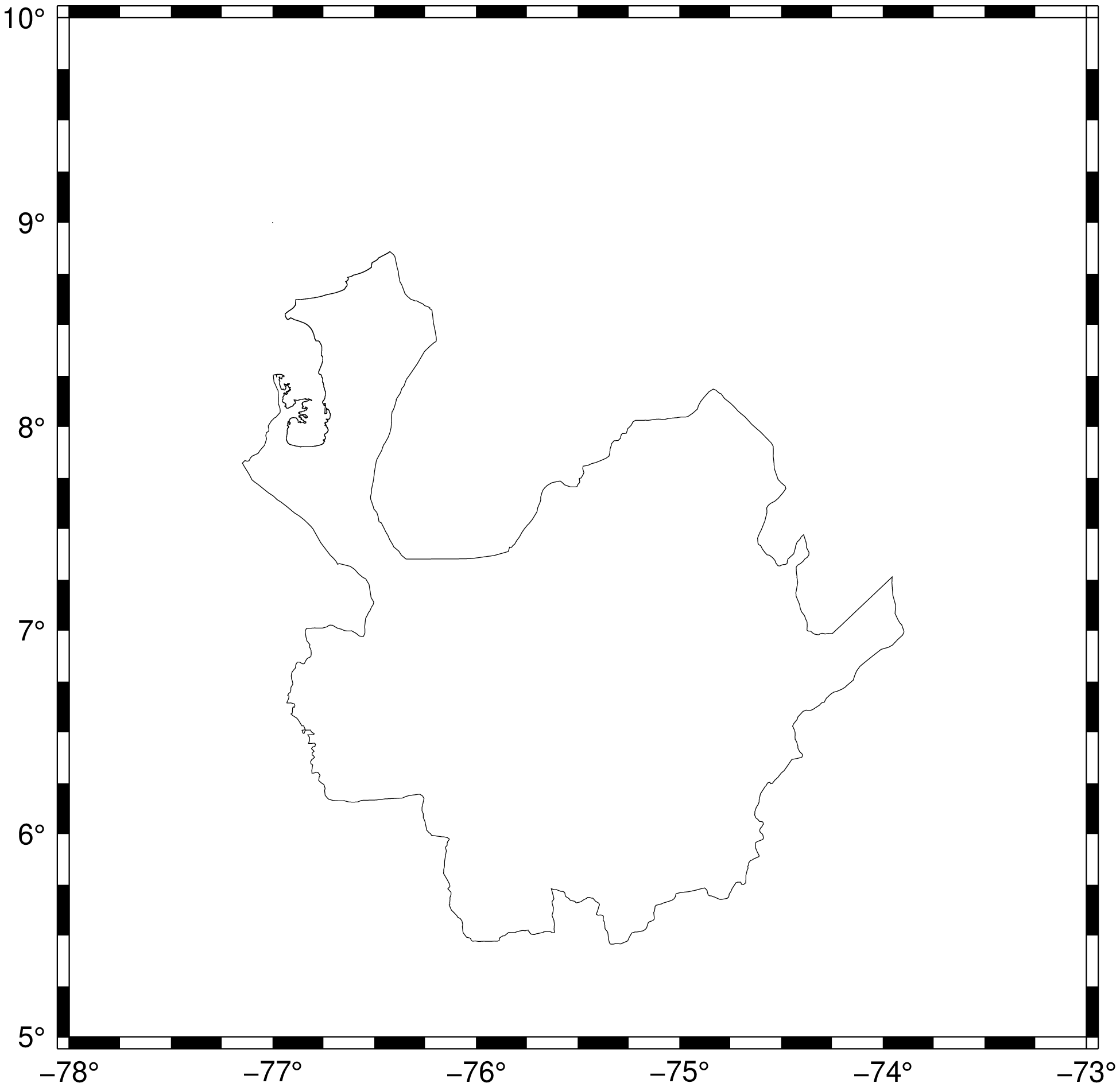
In this demonstration we are interested only in one departament, so we will filter the data to fulfill a department name condition. Review the following code and change it to match your department.
antioquia = filter(deptos, NAME_1 = "Antioquia");Nex, plot the new object.
viz(antioquia, proj=:guess)
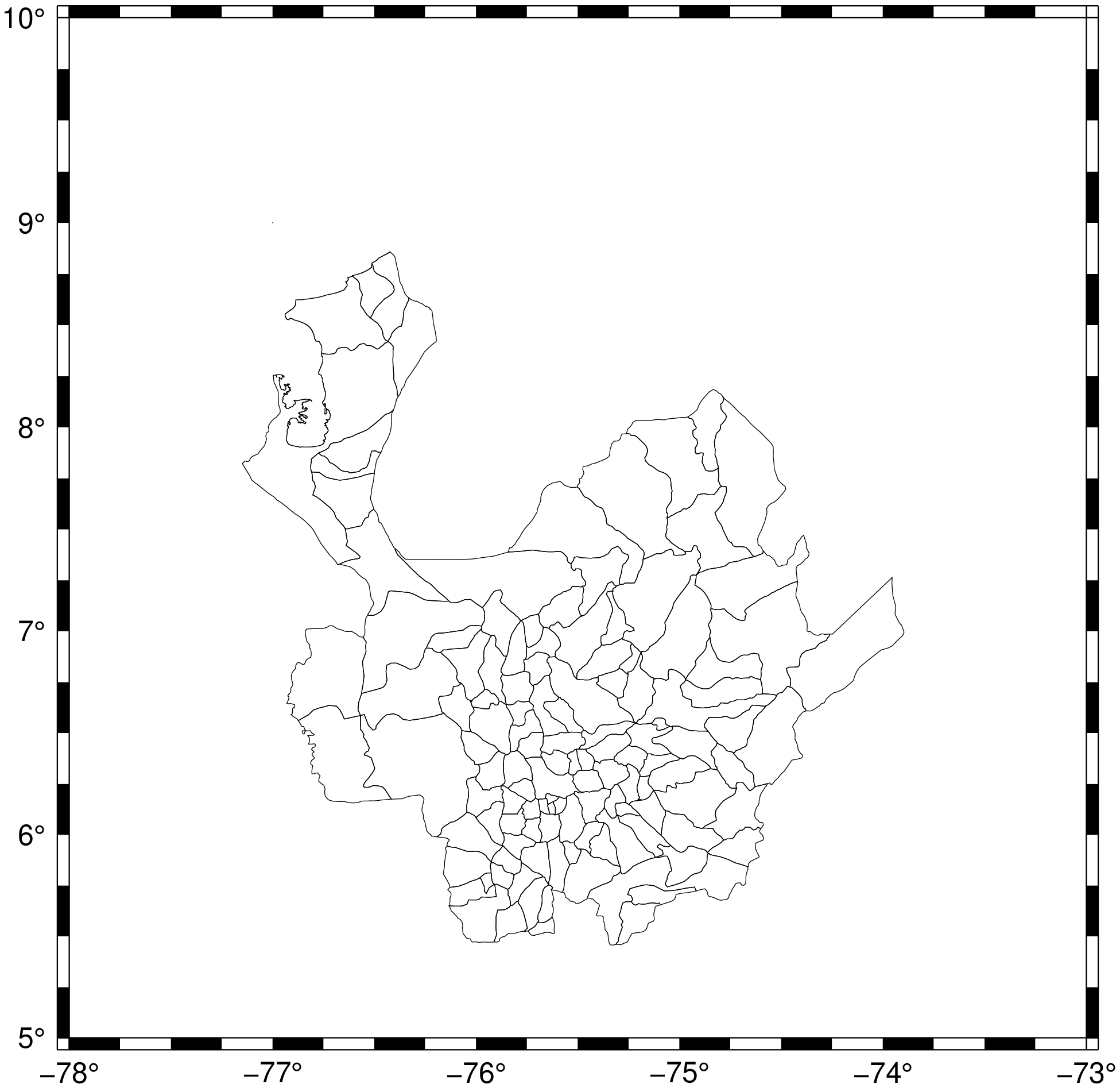
We can repeat the previous steps to load the Colombian municipalities and filter the Antioquian ones.
munic = gmtread(GMT.TESTSDIR * "COL_adm2.shp.zip");
mun_antioquia = filter(munic, NAME_1=:Antioquia);    # Symbols are as good as strings for attribute values
viz(mun_antioquia, proj=:guess)
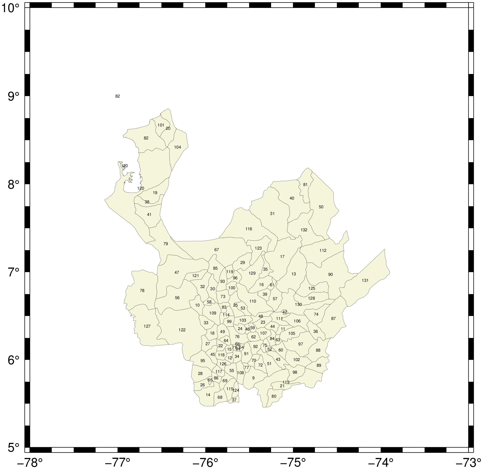
Now we are going to compute the centroids of the Antioquia municipes and use them as placers to contents of the ID_2 attribute (that are numbers, though confess that I don't know what they represent).
antioquia_points = centroid(mun_antioquia);
t = info(mun_antioquia, att="ID_2");        # Get the values of the ID_2 attribute
antioquia_points.text = t;                  # Add the tex column to the centroids object
viz(mun_antioquia, proj=:guess, fill=:beige, lw=0, text=(data=antioquia_points, font=4))
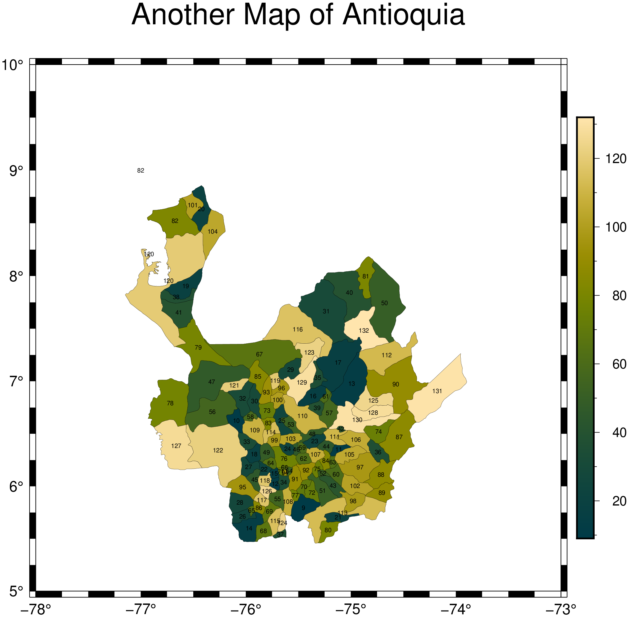
And as an example, we can use the numeric information contained in the ID_2 attribute (which comes out as string but we can easily convert it to numbers) and paint the municipe polygons according to those numbers. That is, make a choropleth map.
# Convert t to numeric. Needed for creating a color map and make the choropleth style plot.
tn = parse.(Int,t);

# Create a color map
C = makecpt(range=(minimum(tn),maximum(tn)), C=:bamako);

# Vizualize
viz(mun_antioquia, proj=:guess, levels=tn, cmap=C, lw=0, title="Another Map of Antioquia", text=(data=antioquia_points, font=5), colorbar=true)
The examples shown here use vector data in the shapefile format, but the same could have been obtained using for example the geopackage format. In fact, as indicated in the SAGA-GIS site from where the shapefiles were downloaded, the original data originates from the GADM project where data was in gpkg format. We can access the data from that site using the gadm function (see examples in GADM). For example, the Antioquia municipes can be downloaded with:
antioquia = gadm("COL", "Antioquia", children=true);But that object does not contain the ID_2 attribute so in fact we couldn't have made the same choropleth map.
These docs were autogenerated using GMT: v1.33.1